TyT2019W30 - Black and White

Get the data

wildlife_impacts <- readr::read_csv("https://raw.githubusercontent.com/rfordatascience/tidytuesday/master/data/2019/2019-07-23/wildlife_impacts.csv")

## Rows: 56978 Columns: 21

## ── Column specification ────────────────────────────────────────────────────────
## Delimiter: ","
## chr  (13): state, airport_id, airport, operator, atype, type_eng, species_id...
## dbl   (7): num_engs, incident_month, incident_year, time, height, speed, cos...
## dttm  (1): incident_date

## 
## ℹ Use `spec()` to retrieve the full column specification for this data.
## ℹ Specify the column types or set `show_col_types = FALSE` to quiet this message.

Explore the data

summary(wildlife_impacts)

##  incident_date                    state            airport_id       
##  Min.   :1990-01-01 00:00:00   Length:56978       Length:56978      
##  1st Qu.:2001-11-15 00:00:00   Class :character   Class :character  
##  Median :2009-11-03 00:00:00   Mode  :character   Mode  :character  
##  Mean   :2008-05-21 04:57:11                                        
##  3rd Qu.:2015-07-26 00:00:00                                        
##  Max.   :2018-12-31 00:00:00                                        
##                                                                     
##    airport            operator            atype             type_eng        
##  Length:56978       Length:56978       Length:56978       Length:56978      
##  Class :character   Class :character   Class :character   Class :character  
##  Mode  :character   Mode  :character   Mode  :character   Mode  :character  
##                                                                             
##                                                                             
##                                                                             
##                                                                             
##   species_id          species             damage             num_engs    
##  Length:56978       Length:56978       Length:56978       Min.   :1.000  
##  Class :character   Class :character   Class :character   1st Qu.:2.000  
##  Mode  :character   Mode  :character   Mode  :character   Median :2.000  
##                                                           Mean   :2.059  
##                                                           3rd Qu.:2.000  
##                                                           Max.   :4.000  
##                                                           NA's   :233    
##  incident_month   incident_year  time_of_day             time      
##  Min.   : 1.000   Min.   :1990   Length:56978       Min.   : -84   
##  1st Qu.: 5.000   1st Qu.:2001   Class :character   1st Qu.: 930   
##  Median : 8.000   Median :2009   Mode  :character   Median :1426   
##  Mean   : 7.235   Mean   :2008                      Mean   :1428   
##  3rd Qu.:10.000   3rd Qu.:2015                      3rd Qu.:1950   
##  Max.   :12.000   Max.   :2018                      Max.   :2359   
##                                                     NA's   :26124  
##      height            speed       phase_of_flt           sky           
##  Min.   :    0.0   Min.   :  0.0   Length:56978       Length:56978      
##  1st Qu.:    0.0   1st Qu.:130.0   Class :character   Class :character  
##  Median :   50.0   Median :140.0   Mode  :character   Mode  :character  
##  Mean   :  983.8   Mean   :154.6                                        
##  3rd Qu.: 1000.0   3rd Qu.:170.0                                        
##  Max.   :25000.0   Max.   :354.0                                        
##  NA's   :18038     NA's   :30046                                        
##     precip          cost_repairs_infl_adj
##  Length:56978       Min.   :      11     
##  Class :character   1st Qu.:    5128     
##  Mode  :character   Median :   26783     
##                     Mean   :  242388     
##                     3rd Qu.:   93124     
##                     Max.   :16380000     
##                     NA's   :56363

Prepare the data

nb_impact<-wildlife_impacts %>%
  mutate(Year=incident_year) %>% 
  select(Year) %>% 
  filter(Year >= 2003 & Year <=2018 & !Year %in% NA)%>%
  group_by(Year)%>% 
  summarise(nb_impact=dplyr::n())


nb_vol<-total_flight %>%
  filter(Year >= 2003 & Year <=2018 & !Year %in% NA) %>% 
  select(Year, TOTAL) %>% 
  left_join(nb_impact,by="Year") %>% 
  mutate(pct=(nb_impact/TOTAL*100))

Visualize the data

#Graphique 
gg<-ggplot(data=nb_vol, aes(x = Year, y=pct))
gg<-gg + geom_bar(stat="identity", position="stack", width=0.80, color="#000505", fill="#000505")
#Ajouter les étiquettes de données 
gg<-gg + geom_text(data=nb_vol, aes(x=Year, y=pct, label=paste0(round(nb_vol$pct,2),"%", sep="")),
                     color=c("#FFFFFF", "#FFFFFF", "#FFFFFF", "#FFFFFF", "#FFFFFF", "#FFFFFF", "#FFFFFF", "#FFFFFF", "#FFFFFF", "#FFFFFF","#FFFFFF", "#FFFFFF", "#FFFFFF","#FFFFFF", "#FFFFFF", "#FFFFFF" ), size=4, vjust=1.6, family="Calibri", fontface="bold")
#ajuster les axes 
gg<-gg + scale_y_continuous(breaks=seq(0,0.05,0.01), limits = c(0, 0.05))
gg<-gg + scale_x_continuous(breaks=seq(2003,2018,1), limits = c(2002.5, 2018.5))
#modifier le thème
gg<-gg +theme(panel.border = element_blank(),
              panel.background = element_blank(),
              plot.background = element_blank(),
              panel.grid.major.y= element_blank(),
              panel.grid.major.x= element_blank(),
              panel.grid.minor = element_blank(),
              axis.line.x = element_blank(),
              axis.line.y = element_blank(),
              axis.ticks.y = element_blank(),
              axis.ticks.x = element_blank())
#ajouter les titres
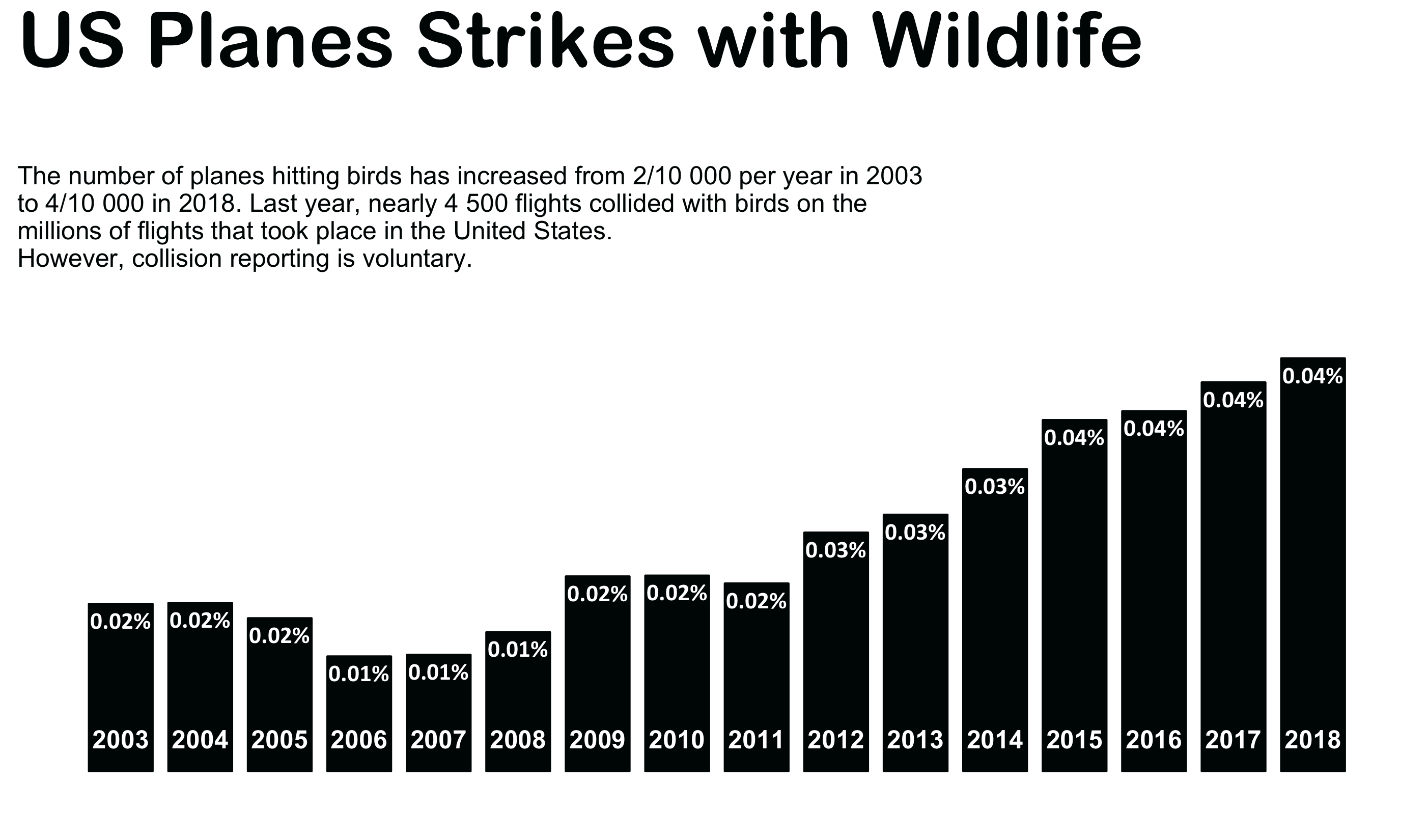
gg<-gg + labs(title="US Planes Strikes with Wildlife\n  ",
              subtitle="The number of planes hitting birds has increased from 2/10 000 per year in 2003\nto 4/10 000 in 2018. Last year, nearly 4 500 flights collided with birds on the\nmillions of flights that took place in the United States.\nHowever, collision reporting is voluntary.",
              y=" ", 
              x=" ")
gg<-gg + theme(plot.title    = element_text(hjust=0,size=36, color="#000505", face="bold", family="Arial Rounded MT Bold"),
               plot.subtitle = element_text(hjust=0,size=12, color="#000505"),
               axis.title.y  = element_blank(),
               axis.title.x  = element_blank(),
               axis.text.y   = element_blank(), 
               axis.text.x   = element_text(hjust=0.5, vjust=15, size=12, color="#FFFFFF", face="bold"))