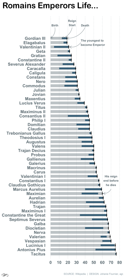
TyT2019W33 - Bullet Graph
By Johanie Fournier, agr. in rstats tidyverse tidytuesday
August 13, 2019
Get the data
emperors <- readr::read_csv("https://raw.githubusercontent.com/rfordatascience/tidytuesday/master/data/2019/2019-08-13/emperors.csv")
## Rows: 68 Columns: 16
## ── Column specification ────────────────────────────────────────────────────────
## Delimiter: ","
## chr  (11): name, name_full, birth_cty, birth_prv, rise, cause, killer, dynas...
## dbl   (1): index
## date  (4): birth, death, reign_start, reign_end
##
## ℹ Use `spec()` to retrieve the full column specification for this data.
## ℹ Specify the column types or set `show_col_types = FALSE` to quiet this message.
Explore the data
summary(emperors)
##      index           name            name_full             birth
##  Min.   : 1.00   Length:68          Length:68          Min.   :0002-12-24
##  1st Qu.:17.75   Class :character   Class :character   1st Qu.:0123-12-13
##  Median :34.50   Mode  :character   Mode  :character   Median :0201-01-01
##  Mean   :34.50                                         Mean   :0184-07-15
##  3rd Qu.:51.25                                         3rd Qu.:0250-01-01
##  Max.   :68.00                                         Max.   :0371-01-01
##                                                        NA's   :5
##      death             birth_cty          birth_prv             rise
##  Min.   :0014-08-19   Length:68          Length:68          Length:68
##  1st Qu.:0189-10-20   Class :character   Class :character   Class :character
##  Median :0251-08-08   Mode  :character   Mode  :character   Mode  :character
##  Mean   :0236-06-01
##  3rd Qu.:0310-09-25
##  Max.   :0395-01-17
##
##   reign_start           reign_end             cause
##  Min.   :0014-09-18   Min.   :0014-08-19   Length:68
##  1st Qu.:0173-01-17   1st Qu.:0189-10-20   Class :character
##  Median :0250-08-08   Median :0251-08-08   Mode  :character
##  Mean   :0228-06-24   Mean   :0236-02-08
##  3rd Qu.:0305-05-01   3rd Qu.:0306-11-06
##  Max.   :0379-01-01   Max.   :0395-01-17
##
##     killer            dynasty              era               notes
##  Length:68          Length:68          Length:68          Length:68
##  Class :character   Class :character   Class :character   Class :character
##  Mode  :character   Mode  :character   Mode  :character   Mode  :character
##
##
##
##
##   verif_who
##  Length:68
##  Class :character
##  Mode  :character
##
##
##
##
Prepare the data
data<-emperors %>%
  mutate(annee_naiss=year(birth)) %>%
  mutate(annee_mort=year(death)) %>%
  mutate(annee_deb=year(reign_start)) %>%
  mutate(annee_fin=year(reign_end)) %>%
  mutate(age_mort=abs(annee_mort-annee_naiss)) %>%
  mutate(age_deb=abs(annee_deb-annee_naiss)) %>%
  mutate(age_fin=abs(annee_fin-annee_naiss)) %>%
  mutate(duree=abs(age_fin-age_deb)) %>%
  mutate(remove=ifelse(age_deb==age_mort, 'retirer', NA)) %>%
  filter(!age_mort %in% NA,!age_deb %in% NA,!age_fin %in% NA,
         !age_mort %in% 4, !remove %in% "retirer") %>%
  select(name, age_deb, age_fin, age_mort, duree)
Visualize the data
#Graphique
gg<-ggplot(data, aes(x=reorder(name, -age_mort), y=age_mort))
gg <- gg + geom_bar(stat="identity", position="stack", width=0.65, fill="#6D7C83", alpha=0.4)
gg <- gg + geom_segment(aes(y = age_deb,
                            x = name,
                            yend = age_fin,
                            xend = name),
                        color = "#175676", size=2.3, alpha=0.8)
gg <- gg + geom_errorbar(aes(y=age_mort, x=name, ymin=age_mort, ymax=age_mort), color="black", width=0.85)
gg <- gg + geom_point(aes(name, age_mort), colour="black", size=0.75)
gg <- gg + coord_flip()
#ajuster les axes
gg <- gg + scale_y_continuous(breaks=seq(0,80,10), limits = c(0,80))
gg <- gg + expand_limits(x=c(0, 56))
#modifier le thème
gg <- gg +  theme(panel.border = element_blank(),
                    panel.background = element_blank(),
                    plot.background = element_blank(),
                    panel.grid.major.x= element_line(size=0.2,linetype="dotted", color="#6D7C83"),
                    panel.grid.major.y= element_blank(),
                    panel.grid.minor = element_blank(),
                    axis.line.x = element_blank(),
                    axis.line.y = element_blank(),
                    axis.ticks.y = element_blank(),
                    axis.ticks.x = element_blank())
#ajouter les titres
gg<-gg + labs(title=" ",
              subtitle="",
              y=" ",
              x=" ")
gg<-gg + theme(plot.title    = element_blank(),
                 plot.subtitle = element_blank(),
                 axis.title.y  = element_blank(),
                 axis.title.x  = element_blank(),
                 axis.text.y   = element_text(hjust=1, vjust=0.5, size=12, color="#6D7C83", face="bold"),
                 axis.text.x   = element_text(hjust=0.5, vjust=0, size=12, color="#6D7C83", face="bold"))
#Faire des flèches
arrows <- tibble(
  x1 = c(50, 16, 53.5, 53.5, 53.5),
  x2 = c(49, 15,   51,   51,   51),
  y1 = c(35, 70,    5,   25,   40),
  y2 = c(22, 61,    0,   13,   19)
)
gg<-gg +    geom_curve(data = arrows, aes(x = x1, y = y1, xend = x2, yend = y2),
                              arrow = arrow(length = unit(0.1, "inch")),
                              size = 0.3, color = "#6D7C83", curvature = -0.3)
#ajouter les étiquettes de données
gg<-gg + annotate(geom="text", x=50,y=35, label="The youngest to\nbecome Emperor", color="#6D7C83", size=3, hjust=0,vjust=0.5, fontface="bold")
gg<-gg + annotate(geom="text", x=18,y=70, label="His reign\nend before\nhe dies", color="#6D7C83", size=3, hjust=0.5,vjust=0.5, fontface="bold")
gg<-gg + annotate(geom="text", x=54,y=5, label="Birth", color="#6D7C83", size=3, hjust=0.5,vjust=0.5, fontface="bold")
gg<-gg + annotate(geom="text", x=55,y=25, label="Reign\nStart", color="#6D7C83", size=3, hjust=0.5,vjust=0.8, fontface="bold")
gg<-gg + annotate(geom="text", x=54,y=40, label="Death", color="#6D7C83", size=3, hjust=0.5,vjust=0.5, fontface="bold")
- Posted on:
- August 13, 2019
- Length:
- 3 minute read, 569 words
- Categories:
- rstats tidyverse tidytuesday
- Tags:
- rstats tidyverse tidytuesday