TyT2019W35 - tvthemes: Les Simpsons

simpsons <- readr::read_delim("https://raw.githubusercontent.com/rfordatascience/tidytuesday/master/data/2019/2019-08-27/simpsons-guests.csv", delim = "|", quote = "")

summary(simpsons)

#Combien y a-t-il de saison?
inspect_season<-simpsons %>%
   inspect_cat()
season<-inspect_season$levels$season %>% 
  filter(!value=="Movie") %>%
 mutate(value=as.numeric(value)) 
#aucune données pour les saisons 15 et 20

#Identifier l'acteur qui revient le plus souvent dans tous les épisodes
simpsons_freq <- simpsons %>%
  inspect_cat()
acteur<-simpsons_freq$levels$guest_star 
#Marcia Wallace

simpsons_cat <- simpsons %>% 
 mutate(season=as.numeric(season)) %>% 
 mutate(acteur=ifelse(guest_star %in% c("Marcia Wallace"),"Marcia Wallace","Autre")) %>% 
 group_by(season, acteur) %>% 
 summarise(nb=dplyr::n()) %>% 
 filter(!season %in% NA) %>% 
 spread(acteur, nb) %>% 
 mutate(`Marcia Wallace`=ifelse(is.na(`Marcia Wallace`), 0, `Marcia Wallace`)) %>% 
 mutate(pct_Marcia=`Marcia Wallace`/(`Marcia Wallace`+Autre)*100) %>% 
 mutate(pct_autre=Autre/(`Marcia Wallace`+Autre)*100) %>% 
 select(season,pct_Marcia,pct_autre) %>% 
 gather(acteur, pourcentage, -season) %>% 
 ungroup() %>% 
 add_row(season=15, acteur="pct_autre", pourcentage=100) %>% 
 add_row(season=20, acteur="pct_autre", pourcentage=100)

#Pour mettre les étiquettes de données seulement sur les valeurs concernant Marcia Wallace
simpson_MW<-simpsons_cat %>% 
  filter(acteur=="pct_Marcia") %>% 
  mutate(pourcentage=ifelse(pourcentage==0, NA, pourcentage))

#Graphique 1: 
#loadfonts()
gg<-ggplot(simpsons_cat, aes(x=season, y=pourcentage, group=acteur, fill=acteur))
gg <- gg + geom_bar(stat="identity", position="stack", width=0.80,color="#FEE8C8", fill="#7199E1" )
gg <- gg + geom_bar(data=simpson_MW, aes(x=season, y=pourcentage, group=acteur, fill=acteur),stat="identity", position="stack", width=0.85,color="#FEE8C8", fill="#FEE8C8")
#ajouter les étiquettes de données
gg<-gg + geom_text(data=simpson_MW, aes(x=season, y=pourcentage, label=paste0(round(simpson_MW$pourcentage,0),"%", sep="")),
                     color="#46732EFF", size=3, position = position_stack(vjust = 0.5), family="Akbar", fontface="bold")
gg<- gg + coord_flip()
#retirer la légende
gg <- gg + theme(legend.position = "none")
#ajuster les axes 
gg <- gg + scale_y_continuous(breaks=seq(0,100,100), limits = c(0, 103), expand = c(0, 0), labels = function(x) paste0(x, "%"))
gg <- gg + scale_x_continuous(breaks=seq(1,30,1), limits = c(0, 31), expand = c(0, 0))
#modifier le thème
gg <- gg +  theme(panel.border = element_blank(),
                    panel.background = element_rect(fill="#7199E1"),
                    plot.background = element_rect(fill ="#7199E1"),
                    panel.grid.major.x= element_blank(),
                    panel.grid.major.y= element_blank(),
                    panel.grid.minor = element_blank(),
                    axis.line.x = element_blank(),
                    axis.line.y = element_blank(),
                    axis.ticks.y = element_blank(),
                    axis.ticks.x = element_blank())
#ajouter les titres
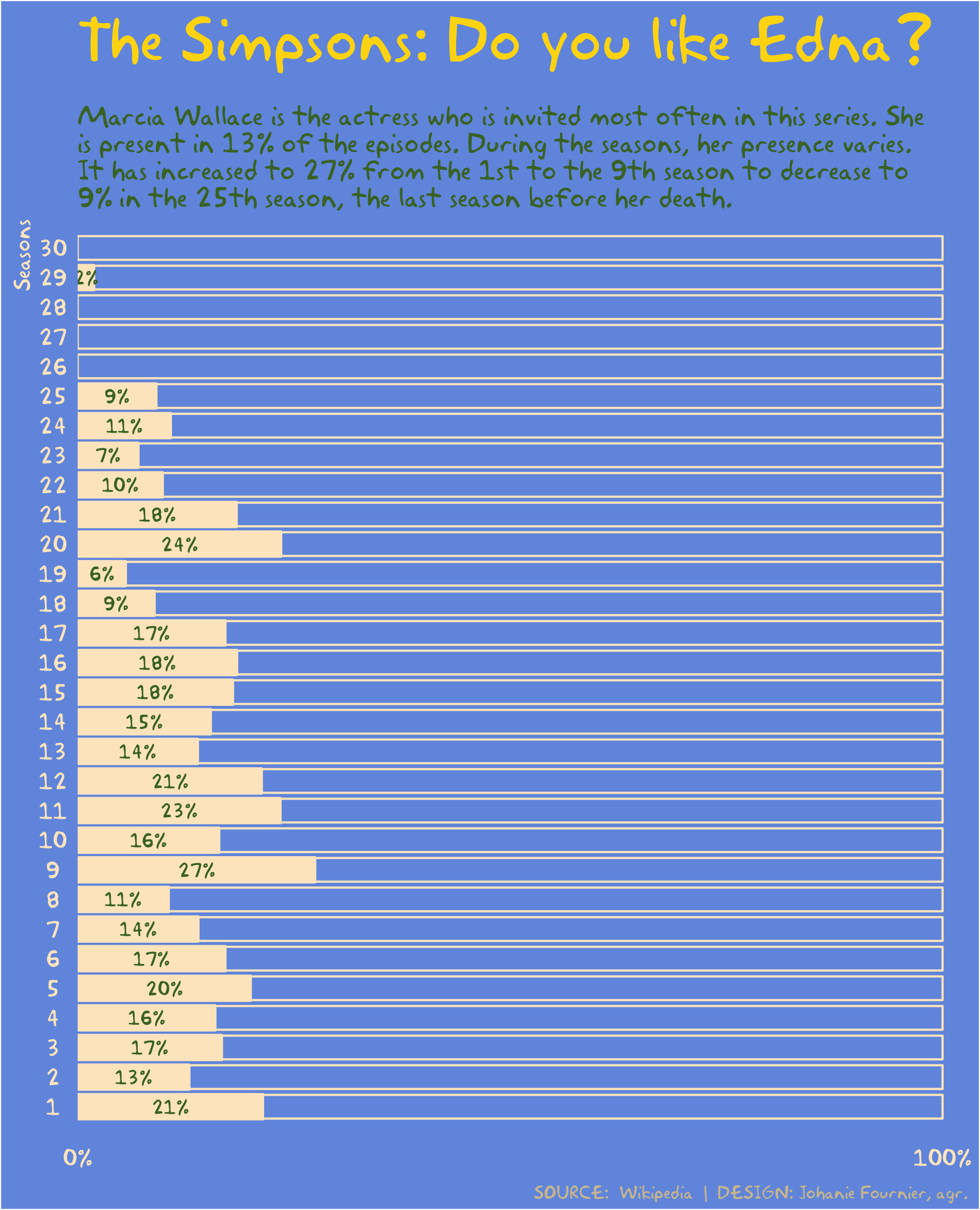
gg<-gg + labs(title="The Simpsons: Do you like Edna?",
              subtitle="\nMarcia Wallace is the actress who is invited most often in this series. She\nis present in 13% of the episodes. During the seasons, her presence varies.\nIt has increased to 27% from the 1st to the 9th season to decrease to\n9% in the 25th season, the last season before her death.",
              x="Seasons", 
              y=" ", 
              caption="SOURCE:  Wikipedia  |  DESIGN: Johanie Fournier, agr.")
gg<-gg + theme(plot.title      = element_text(size=27, hjust=0,vjust=0, face="bold", family="Akbar", color="#fed90f"),
                 plot.subtitle = element_text(size=12, hjust=0,vjust=0, family="Akbar", color="#46732EFF"),
                 plot.caption =  element_text(size=8, hjust=1,vjust=0, family="Akbar", color="#D1C19E"),
                 axis.title.y  = element_text(size=10, hjust=1,vjust=0.5, family="Akbar", color="#FEE8C8"),
                 axis.title.x  = element_blank(),
                 axis.text.x   = element_text(size=10, hjust=0.5,vjust=0.5, family="Akbar", color="#FEE8C8"), 
                 axis.text.y   = element_text(size=10, hjust=0.5,vjust=0.5, family="Akbar", color="#FEE8C8"))