TyT2019W37 - Two Graphs for a Summary

tx_injuries <- readr::read_csv("https://raw.githubusercontent.com/rfordatascience/tidytuesday/master/data/2019/2019-09-10/tx_injuries.csv")

#code<-read.csv('~/Documents/ENTREPRISE/Projets R/Tidytuesday/codes_us.csv', header = TRUE, sep=";")

summary(tx_injuries)

# Corriger le format des dates
data<-tx_injuries %>% 
mutate(janitor_date = as.numeric(injury_date) %>%
       janitor::excel_numeric_to_date(.),
       lubridate_date = lubridate::mdy(injury_date),
       real_date = coalesce(janitor_date, lubridate_date)) %>%
  select(-injury_date,
         -janitor_date,
         -lubridate_date) %>% 
  unnest_tokens(word, body_part) %>%
  anti_join(stop_words) %>%
filter(!is.na(real_date),!is.na(word), !gender %in% c("N/A", "n/a")) %>% 
  select(real_date, word, gender, st) %>% 
  mutate(annee=year(real_date), mois=month(real_date)) 

#Données pour le premier graphique:
by_country<-data %>% 
  mutate(Abbreviation=st) %>% 
  left_join(code, by="Abbreviation") %>% 
  filter(!State %in% c("Arizona", "Florida")) %>% 
  select(-st, -Abbreviation, -gender, -word) %>% 
  group_by(mois, annee) %>% 
  summarise(nb=dplyr::n()) 
  
  
#Données pour le deuxième graphique:
blessure <- data %>%
    group_by(gender, word) %>% 
    summarise(nb=dplyr::n()) %>%
    ungroup() %>% 
    mutate(gender=ifelse(gender=="m", "M", gender)) %>% 
    filter(gender %in% c("M", "F"))%>% 
  filter(word %in% c("head", "shoulder", "neck", "ankle", "elbow", "foot", "arm", "mouth", "forearm")) #%>% 
  #mutate(word=ifelse(word=="head","Tête",word))%>%
 # mutate(word=ifelse(word=="shoulder","Épaule",word))%>%
 # mutate(word=ifelse(word=="neck","Cou",word))%>%
 # mutate(word=ifelse(word=="ankle","Cheville",word))%>%
 # mutate(word=ifelse(word=="elbow","Coude",word))%>%
 # mutate(word=ifelse(word=="foot","Pied",word))%>%
 # mutate(word=ifelse(word=="arm","Bras",word))%>%
 # mutate(word=ifelse(word=="mouth","Bouche",word))%>%
 # mutate(word=ifelse(word=="forearm","Avant-Bras",word))

blessure_h <- blessure
blessure_h$nb <- ifelse(blessure_h$gender == "F", blessure_h$nb  * -1, blessure_h$nb)

#Créer le titre
couleur <- image_read('~/Documents/ENTREPRISE/Projets R/couleur/38607A.png')
titre<- couleur %>%
  image_scale("x20") %>% 
  image_background("#38607A", flatten = TRUE) %>%
  image_border("#38607A", "500x90") %>% 
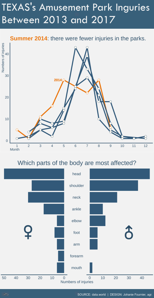
  image_annotate("Incidents des parcs d'attractions\nau TEXAS entre 2013 et 2017",
                 color = "#F5F5F5", size = 80, location = "+10+5", font='Tw Cen MT') 
#image_browse(titre)


#Graphique plot 1
gg<-ggplot(by_country, aes(x=factor(mois), y=nb, group=annee, color=factor(annee)))
gg<-gg + geom_line(size = 2, show.legend = F) 
gg<-gg + geom_point(shape = 21, fill = "#FFFBF4", size = 4, show.legend = F) 
gg<-gg + scale_color_manual(values = c("#406D8C", "#F08805", "#406D8C", "#406D8C", "#406D8C"))
#étiquette
gg <- gg +  geom_text(aes(y = 28, x = 4.5),label = "2014", size = 5, family = "Tw Cen MT",  color="#F08805", hjust=0.5, fontface="bold")
#modifier le thème
gg <- gg +  theme(panel.border = element_blank(),
                    panel.background = element_rect(fill="#F5F5F5"),
                    plot.background = element_rect(fill ="#F5F5F5"),
                    panel.grid.major.x= element_blank(),
                    panel.grid.major.y= element_blank(),
                    panel.grid.minor = element_blank(),
                    axis.line.x = element_line(size=1, color="#38607A"),
                    axis.line.y = element_line(size=1, color="#38607A"),
                    axis.ticks = element_blank())
#ajouter les titres
gg<-gg + labs(title="<br><span style='color:#F08805'>**Été 2014**</span><span style='color:#38607A'>: il y a eu moins d'incidents dans les parcs.</span>",
              y="nombre d'incidents", 
              x="Mois")
gg<-gg + theme(  plot.title    = element_markdown(lineheight = 1.1,size=23.5, hjust=0,vjust=0, family="Tw Cen MT"),
                 axis.title.y  = element_text(size=14, hjust=1,vjust=0.5, family="Tw Cen MT", color="#38607A"),
                 axis.title.x  = element_text(size=14, hjust=0,vjust=0.5, family="Tw Cen MT", color="#38607A"),
                 axis.text.x   = element_text(size=14, hjust=0.5,vjust=0.5, family="Tw Cen MT", color="#38607A"), 
                 axis.text.y   = element_text(size=14, hjust=0.5,vjust=0.5, family="Tw Cen MT", color="#38607A"))


#Graphique plot 2
female = intToUtf8(9792)
male = intToUtf8(9794)

gg<-ggplot(data=blessure_h, aes(x=reorder(word,desc(-abs(nb))), y=nb, fill=gender)) 
gg<-gg + geom_bar(stat = "identity", show.legend = F) 
gg<-gg + facet_share(~gender, dir = "h", scales = "free", reverse_num = TRUE) 
gg<-gg + coord_flip() 
gg<-gg + scale_fill_manual(values = c("#406D8C", "#406D8C"))
#retirer les titres du facet_wrap
gg<-gg + theme(strip.background = element_blank(),
               strip.text.x = element_blank())
#Ajouter des étiquettes
gg<-gg + geom_text(x = 4, y = -30, label = female, hjust = 0.5, size = 25, color = "#38607A",family = "Tw Cen MT", fontface = "bold") 
gg<-gg +   geom_text(x = 4, y = 30, label = male, hjust = 0.5, size = 25, color = "#38607A", family = "Tw Cen MT", fontface = "bold")
#modifier le thème
gg <- gg +  theme(panel.border = element_blank(),
                    panel.background = element_rect(fill="#F5F5F5"),
                    plot.background = element_rect(fill ="#F5F5F5"),
                    panel.grid.major.x= element_blank(),
                    panel.grid.major.y= element_blank(),
                    panel.grid.minor = element_blank(),
                    axis.line.x = element_line(size=1, color="#38607A"),
                    axis.line.y = element_line(size=1, color="#38607A"),
                    axis.ticks = element_blank())
#ajouter les titres
gg<-gg + labs(title="\nQuelles sont les parties du corps les plus touchées ?",
              y="nombre d'incidents\n")
gg<-gg + theme(  plot.title    = element_text(size=23, hjust=0.5,vjust=0.5, family="Tw Cen MT", color="#38607A"),
                 axis.title.x  = element_text(size=14, hjust=0.5,vjust=0.5, family="Tw Cen MT", color="#38607A"),
                 axis.title.y  = element_blank(),
                 axis.text.x   = element_text(size=14, hjust=0.5,vjust=0.5, family="Tw Cen MT", color="#38607A"), 
                 axis.text.y   = element_text(size=14, hjust=0.5,vjust=0.5, family="Tw Cen MT", color="#38607A"))


# And bring in a logo
logo_raw<-image_read('~/Documents/ENTREPRISE/Projets R/Logo/Logo_gris_38607A.png')
logo <- logo_raw %>%
  image_scale("x30") %>% 
  image_background("#38607A", flatten = TRUE) %>%
  image_border("#38607A", "10x10")

couleur <- image_read('~/Documents/ENTREPRISE/Projets R/couleur/38607A.png')
backgound <- couleur %>%
  image_scale("x20") %>% 
  image_background("#38607A", flatten = TRUE) %>%
  image_border("#38607A", "500x20")
  
footer<-image_composite(backgound, logo, offset="+0+10") %>% 
  image_annotate("SOURCE: data.world  |  DESIGN: Johanie Fournier, agr.",
                 color = "#F5F5F5", size = 20, gravity='northeast', location = "+10+25")
#image_browse(footer)

# Stack them on top of each other
final_plot <- image_append(image_scale(c(titre,plot1,plot2, footer),"500"), stack = TRUE)