TyT2019W38 - When Your Data Form a Tree!
By Johanie Fournier, agr. in rstats tidyverse tidytuesday
September 20, 2019
Get the data
park_visits <- readr::read_csv("https://raw.githubusercontent.com/rfordatascience/tidytuesday/master/data/2019/2019-09-17/national_parks.csv")
## Rows: 21560 Columns: 12
## ── Column specification ────────────────────────────────────────────────────────
## Delimiter: ","
## chr (9): year, geometry, metadata, parkname, region, state, unit_code, unit_...
## dbl (3): gnis_id, number_of_records, visitors
##
## ℹ Use `spec()` to retrieve the full column specification for this data.
## ℹ Specify the column types or set `show_col_types = FALSE` to quiet this message.
Explore the data
summary(park_visits)
## Warning: One or more parsing issues, see `problems()` for details
##      year              gnis_id          geometry           metadata
##  Length:21560       Min.   :   2877   Length:21560       Length:21560
##  Class :character   1st Qu.: 401309   Class :character   Class :character
##  Mode  :character   Median :1009494   Mode  :character   Mode  :character
##                     Mean   :1070863
##                     3rd Qu.:1530459
##                     Max.   :2775865
##                     NA's   :2
##  number_of_records   parkname            region             state
##  Min.   :1         Length:21560       Length:21560       Length:21560
##  1st Qu.:1         Class :character   Class :character   Class :character
##  Median :1         Mode  :character   Mode  :character   Mode  :character
##  Mean   :1
##  3rd Qu.:1
##  Max.   :1
##
##   unit_code          unit_name          unit_type            visitors
##  Length:21560       Length:21560       Length:21560       Min.   :        0
##  Class :character   Class :character   Class :character   1st Qu.:    39125
##  Mode  :character   Mode  :character   Mode  :character   Median :   155219
##                                                           Mean   :  1277105
##                                                           3rd Qu.:   608144
##                                                           Max.   :871922828
##                                                           NA's   :4
Prepare the data
regions<-park_visits %>%
  select('region') %>%
  inspect_cat() %>%
  show_plot()

year<-park_visits %>%
  select('year') %>%
  inspect_cat()
Visualize the data
#Graphique
gg<-ggplot(data, aes(x=year, y=diff, group=region))
gg<-gg + geom_point(size=1.5,color="#ACC6AB")
gg<-gg + geom_line(size=0.5,color="#C3BDB5")
gg<-gg + geom_point(data=data_m, size=3.5,color="#8EB18C")
gg<-gg + geom_line(data=data_m, size=1.5,color="#5B5144")
gg<-gg + geom_hline(yintercept=0, linetype="dashed", color="#A9A9A9")
#ajuster les axes
gg<-gg + scale_y_continuous(breaks=seq(-40,40,10), limits=c(-40, 40))
gg<-gg + coord_flip()
#modifier le thème
gg <- gg + theme(panel.border = element_blank(),
panel.background = element_blank(),
plot.background = element_blank(),
panel.grid.major.x= element_blank(),
panel.grid.major.y= element_blank(),
panel.grid.minor = element_blank(),
axis.line.x = element_line(size=1, color="#A9A9A9"),
axis.line.y = element_blank(),
axis.ticks = element_blank())
#ajouter les titres
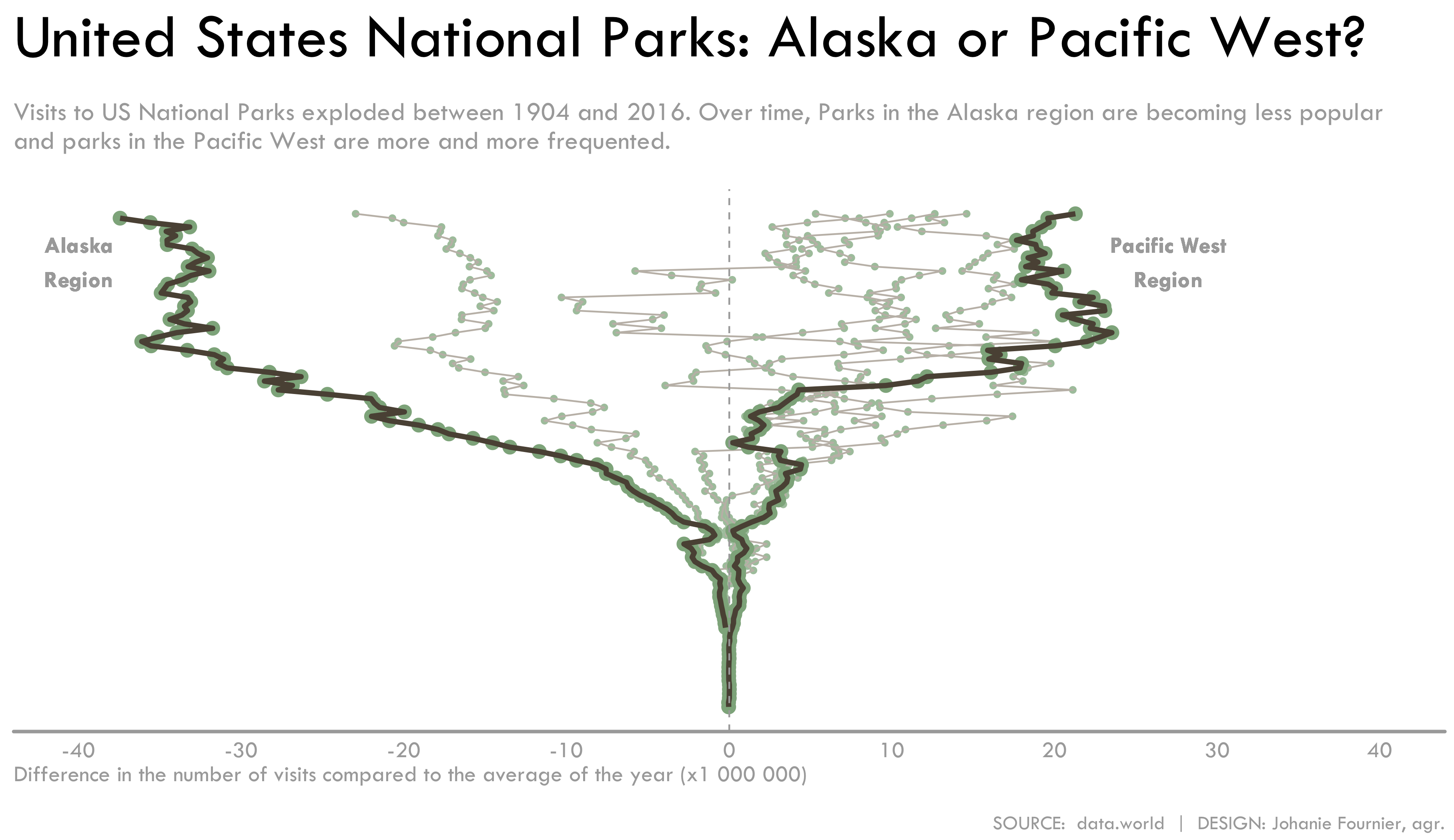
gg<-gg + labs(title="United States National Parks: Alaska or Pacific West?",
subtitle = "\nVisits to US National Parks exploded between 1904 and 2016. Over time, Parks in the Alaska region are becoming less popular\nand parks in the Pacific West are more and more frequented.\n",
x=" ",
y="Difference in the number of visits compared to the average of the year (x1 000 000)",
caption="\nSOURCE: data.world | DESIGN: Johanie Fournier, agr.")
gg<-gg + theme( plot.title = element_text(size=38, hjust=0,vjust=0.5, family="Tw Cen MT", color="black"),
plot.subtitle = element_text(size=16, hjust=0,vjust=0.5, family="Tw Cen MT", color="#A9A9A9"),
plot.caption = element_text(size=12, hjust=1,vjust=0.5, family="Tw Cen MT", color="#A9A9A9"),
axis.title.y = element_blank(),
axis.title.x = element_text(size=14, hjust=0,vjust=0.5, family="Tw Cen MT", color="#A9A9A9"),
axis.text.x = element_text(size=14, hjust=0.5,vjust=0.5, family="Tw Cen MT", color="#A9A9A9"),
axis.text.y = element_blank())
- Posted on:
- September 20, 2019
- Length:
- 2 minute read, 414 words
- Categories:
- rstats tidyverse tidytuesday
- Tags:
- rstats tidyverse tidytuesday