TyT2019W40 - Facet_wrap with dots and lines
By Johanie Fournier, agr. in rstats tidyverse tidytuesday
October 2, 2019
Get the data
pizza_jared <- readr::read_csv("https://raw.githubusercontent.com/rfordatascience/tidytuesday/master/data/2019/2019-10-01/pizza_jared.csv")
## Rows: 375 Columns: 9
## ── Column specification ────────────────────────────────────────────────────────
## Delimiter: ","
## chr (3): answer, question, place
## dbl (6): polla_qid, votes, pollq_id, time, total_votes, percent
##
## ℹ Use `spec()` to retrieve the full column specification for this data.
## ℹ Specify the column types or set `show_col_types = FALSE` to quiet this message.
Explore the data
summary(pizza_jared)
##    polla_qid        answer              votes           pollq_id
##  Min.   : 2.00   Length:375         Min.   : 0.000   Min.   : 2.00
##  1st Qu.:21.00   Class :character   1st Qu.: 0.000   1st Qu.:21.00
##  Median :40.00   Mode  :character   Median : 2.000   Median :40.00
##  Mean   :39.93                      Mean   : 2.832   Mean   :39.93
##  3rd Qu.:59.00                      3rd Qu.: 4.000   3rd Qu.:59.00
##  Max.   :77.00                      Max.   :26.000   Max.   :77.00
##
##    question            place                time            total_votes
##  Length:375         Length:375         Min.   :1.344e+09   Min.   : 0.00
##  Class :character   Class :character   1st Qu.:1.395e+09   1st Qu.: 7.00
##  Mode  :character   Mode  :character   Median :1.467e+09   Median :12.00
##                                        Mean   :1.459e+09   Mean   :14.16
##                                        3rd Qu.:1.519e+09   3rd Qu.:19.00
##                                        Max.   :1.569e+09   Max.   :67.00
##
##     percent
##  Min.   :0.0000
##  1st Qu.:0.0000
##  Median :0.1667
##  Mean   :0.2000
##  3rd Qu.:0.3333
##  Max.   :1.0000
##  NA's   :5
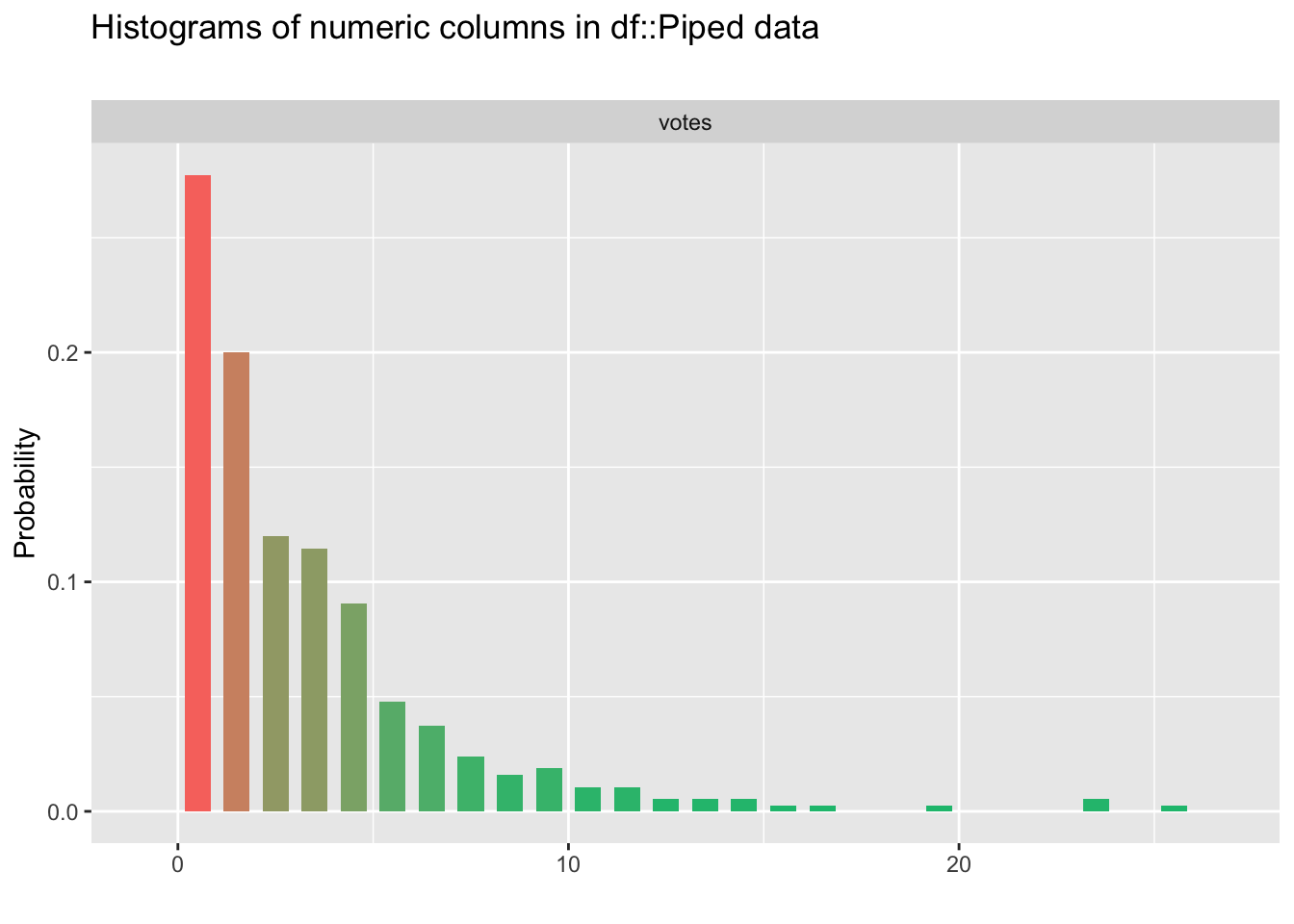
votes<-pizza_jared %>%
  select('votes') %>%
  inspect_num()
show_plot(votes)
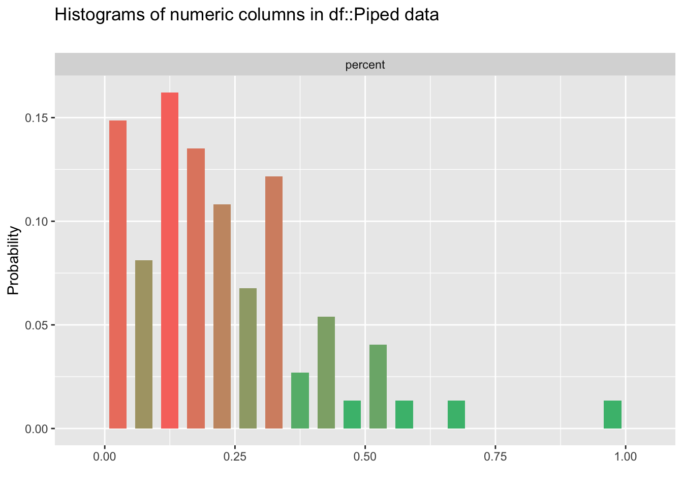
votes<-pizza_jared %>%
  filter(answer=="Excellent") %>%
  select('percent') %>%
  inspect_num()
show_plot(votes)
Prepare the data
excellent<-pizza_jared %>%
    filter(answer=="Excellent" & percent>=0.5) %>%
    select('place') %>%
    distinct()


pizza_jared_top<-pizza_jared %>%
  right_join(excellent, by="place") %>%
  group_by(place, answer) %>%
  summarise(votes_corr=mean(votes))
## `summarise()` has grouped output by 'place'. You can override using the `.groups` argument.
pizza_jared_top$answer <-factor(pizza_jared_top$answer, levels = c("Excellent", "Good", "Average", "Poor", "Never Again"))
pizza_jared_top$place <-factor(pizza_jared_top$place, levels = c( "Prince Street Pizza",  "Patsy's", "Naples 45", "Tappo","Little Italy Pizza", "Fiore's"))

pizza_jared_top<-pizza_jared_top %>%
  mutate(answer=case_when(answer == 'Excellent' ~ "Excellent",
                          answer == 'Good' ~ "Bon",
                          answer == 'Average' ~ "Moyen",
                          answer == 'Poor' ~ "Mauvais",
                          answer == 'Never Again' ~ "Plus Jamais"))

pizza_jared_top$answer <-factor(pizza_jared_top$answer, levels = c("Excellent", "Bon", "Moyen", "Mauvais", "Plus Jamais"))
Visualize the data
#Graphique
gg<-ggplot(pizza_jared_top, aes(x=votes_corr, y=place, color=answer))
gg<-gg + geom_point(size=11, alpha=0.9)
gg<-gg + facet_grid(. ~ answer)
gg<-gg + scale_color_brewer(palette="Set1")
#retier la légende
gg<-gg + theme(legend.position = "none")
#ajuster les axes
gg<-gg + scale_x_continuous(breaks=seq(0,10,2), limits=c(-2, 12))
#Ajouter les étiquettes de données
gg<-gg + geom_text(data=pizza_jared_top, aes(x=votes_corr, y=place, label=(round(pizza_jared_top$votes_corr,0))), color="#5D5D5D", size=5.5, vjust=0.5, hjust=0.5, family="Tw Cen MT", fontface="bold")
#modifier le thème
gg <- gg + theme(panel.border = element_blank(),
panel.background = element_blank(),
plot.background = element_blank(),
panel.grid.major.x= element_blank(),
panel.grid.major.y= element_line(size=1, linetype = "solid", color="#A9A9A9"),
panel.grid.minor = element_blank(),
axis.line.x = element_blank(),
axis.line.y = element_blank(),
axis.ticks = element_blank(),
strip.background =element_blank())
#ajouter les titres
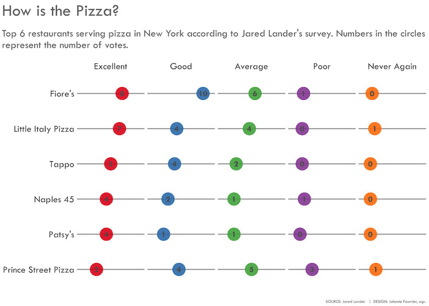
gg<-gg + labs(title="How is the pizza?",
subtitle = "\nTop 6 restaurants serving pizza in New York according to Jared Lander's survey\n",
x=" ",
y=" ",
caption="\nSOURCE: Jared Lander | DESIGN: Johanie Fournier, agr.")
gg<-gg + theme( plot.title = element_blank(),
plot.subtitle = element_blank(),
plot.caption = element_text(size=8, hjust=1,vjust=0.5, family="Tw Cen MT", color="#5D5D5D"),
axis.title.y = element_blank(),
axis.title.x = element_blank(),
axis.text.y = element_text(size=18, hjust=1,vjust=0.5, family="Tw Cen MT", color="#5D5D5D"),
axis.text.x = element_blank(),
strip.text = element_text(size=18, hjust=0.5,vjust=0.5, family="Tw Cen MT", color="#5D5D5D"))
- Posted on:
- October 2, 2019
- Length:
- 3 minute read, 482 words
- Categories:
- rstats tidyverse tidytuesday
- Tags:
- rstats tidyverse tidytuesday