TyT2019W41 - Ratios to compare
By Johanie Fournier, agr. in rstats tidyverse tidytuesday
October 10, 2019
Get the data
ipf_lifts <- readr::read_csv("https://raw.githubusercontent.com/rfordatascience/tidytuesday/master/data/2019/2019-10-08/ipf_lifts.csv")
## Rows: 41152 Columns: 16
## ── Column specification ────────────────────────────────────────────────────────
## Delimiter: ","
## chr  (10): name, sex, event, equipment, age_class, division, weight_class_kg...
## dbl   (5): age, bodyweight_kg, best3squat_kg, best3bench_kg, best3deadlift_kg
## date  (1): date
##
## ℹ Use `spec()` to retrieve the full column specification for this data.
## ℹ Specify the column types or set `show_col_types = FALSE` to quiet this message.
Explore the data
summary(ipf_lifts)
##      name               sex               event            equipment
##  Length:41152       Length:41152       Length:41152       Length:41152
##  Class :character   Class :character   Class :character   Class :character
##  Mode  :character   Mode  :character   Mode  :character   Mode  :character
##
##
##
##
##       age         age_class           division         bodyweight_kg
##  Min.   : 0.50   Length:41152       Length:41152       Min.   : 37.29
##  1st Qu.:22.50   Class :character   Class :character   1st Qu.: 60.00
##  Median :31.50   Mode  :character   Mode  :character   Median : 75.55
##  Mean   :34.77                                         Mean   : 81.15
##  3rd Qu.:45.00                                         3rd Qu.: 97.30
##  Max.   :93.50                                         Max.   :240.00
##  NA's   :2906                                          NA's   :187
##  weight_class_kg    best3squat_kg    best3bench_kg    best3deadlift_kg
##  Length:41152       Min.   :-210.0   Min.   :-160.0   Min.   :-215.0
##  Class :character   1st Qu.: 160.0   1st Qu.:  97.5   1st Qu.: 170.0
##  Mode  :character   Median : 215.0   Median : 140.0   Median : 222.5
##                     Mean   : 217.6   Mean   : 144.7   Mean   : 221.8
##                     3rd Qu.: 270.0   3rd Qu.: 185.0   3rd Qu.: 270.0
##                     Max.   : 490.0   Max.   : 415.0   Max.   : 420.0
##                     NA's   :13698    NA's   :2462     NA's   :14028
##     place                date             federation         meet_name
##  Length:41152       Min.   :1973-11-09   Length:41152       Length:41152
##  Class :character   1st Qu.:1998-12-11   Class :character   Class :character
##  Mode  :character   Median :2007-10-14   Mode  :character   Mode  :character
##                     Mean   :2006-02-19
##                     3rd Qu.:2015-06-05
##                     Max.   :2019-08-26
##
Prepare the data
comp_poids<-ipf_lifts %>%
  mutate(ratio=best3deadlift_kg/bodyweight_kg) %>%
  filter(!is.na(ratio), !is.na(age_class), !age_class=="5-12") %>%
  select(age_class, sex, ratio) %>%
  group_by(sex, age_class) %>%
  summarise(moyenne=mean(ratio, na.rm=TRUE), et=sd(ratio, na.rm=TRUE)) %>%
  mutate(age_class=as.factor(age_class))
## `summarise()` has grouped output by 'sex'. You can override using the `.groups` argument.
Visualize the data
#Graphique
gg<-ggplot(data=comp_poids)
gg<-gg + geom_rect(data=comp_poids, aes(x=age_class, y=moyenne),
xmin=as.numeric(comp_poids$age_class[[5]])-0.5,
xmax=as.numeric(comp_poids$age_class[[6]])+0.5,
ymin=0,
ymax=4,
fill="#E7E7E7", alpha=0.6)
gg<-gg + geom_rect(data=comp_poids, aes(x=age_class, y=moyenne),
xmin=as.numeric(comp_poids$age_class[[9]])-0.5,
xmax=as.numeric(comp_poids$age_class[[10]])+0.5,
ymin=0,
ymax=4,
fill="#E7E7E7", alpha=0.6)
gg<-gg + geom_rect(data=comp_poids, aes(x=age_class, y=moyenne),
xmin=as.numeric(comp_poids$age_class[[12]])-0.5,
xmax=as.numeric(comp_poids$age_class[[13]])+0.5,
ymin=0,
ymax=4,
fill="#E7E7E7", alpha=0.6)
gg<-gg + geom_segment( aes(x=as.numeric(comp_poids$age_class[[5]]),xend=as.numeric(comp_poids$age_class[[13]]),
y=3.24,
yend=2.2),
color="#EA9010", alpha=0.6)
gg<-gg + geom_segment( aes(x=as.numeric(comp_poids$age_class[[5]]),xend=as.numeric(comp_poids$age_class[[13]]),
y=2.73,
yend=1.92),
color="#4A0D67", alpha=0.6)
gg<-gg + geom_point(data=comp_poids,aes(x=age_class, y=moyenne, group=sex, color=sex), size=4.5)
gg<-gg + geom_errorbar(data=comp_poids, aes(x=age_class, ymin=moyenne-et, ymax=moyenne+et, color=sex), width=0.3, size=0.6, alpha=0.6)
gg<-gg + scale_color_manual(values=c("#4A0D67","#EA9010"))
#retier la légende
gg<-gg + theme(legend.position = "none")
#ajuster les axes
gg<-gg + scale_y_continuous(breaks=seq(0,4,0.5), limits=c(0, 4))
#modifier le thème
gg <- gg + theme(panel.border = element_blank(),
panel.background = element_blank(),
plot.background = element_blank(),
panel.grid.major.x= element_blank(),
panel.grid.major.y= element_blank(),
panel.grid.minor = element_blank(),
axis.line.x = element_line(size=0.5, color="#A9A9A9"),
axis.line.y =element_line(size=0.5, color="#A9A9A9"),
axis.ticks = element_blank())
#ajouter les titres
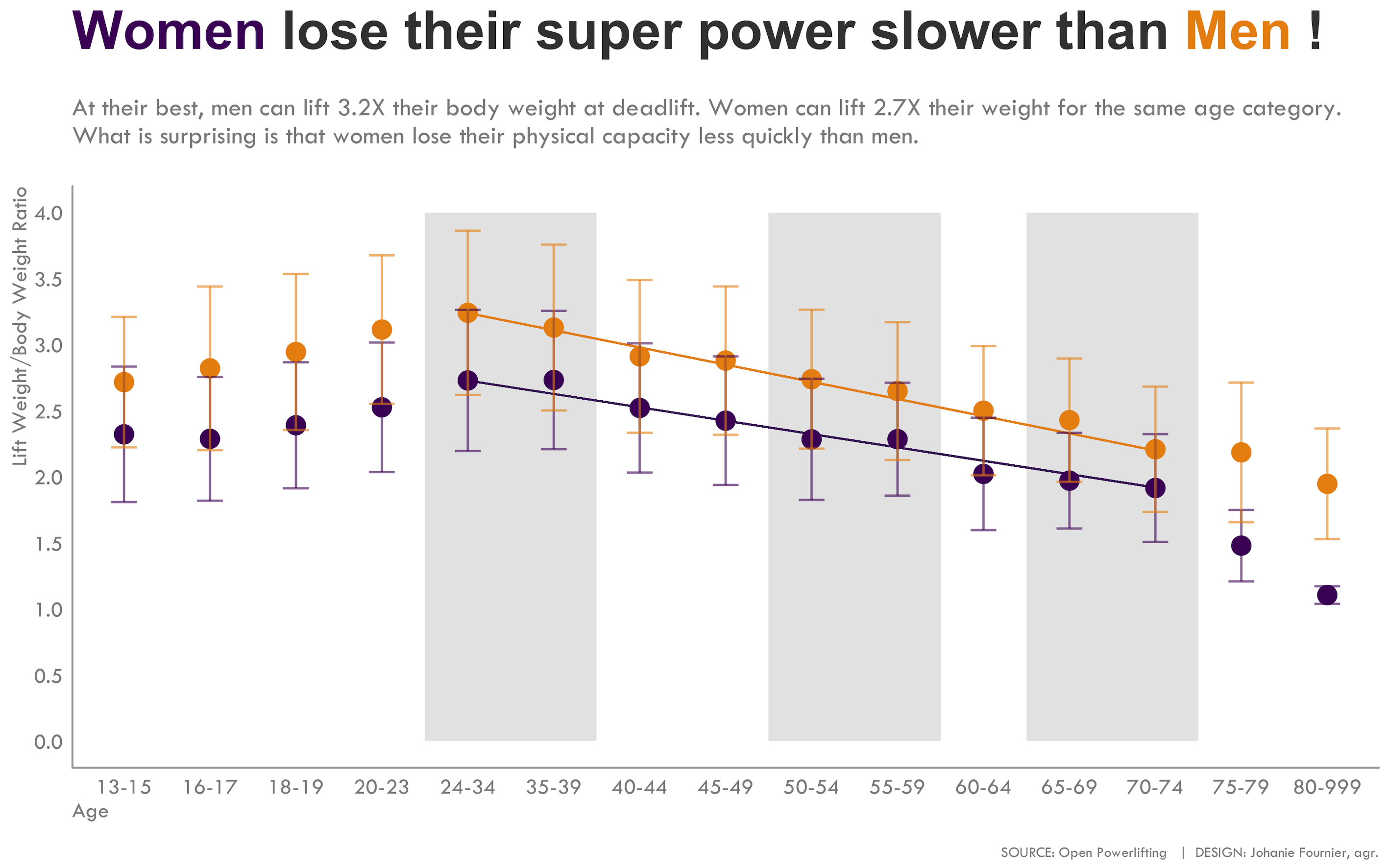
gg<-gg + labs(title="<span style='color:#4A0D67'>**Women**</span> lose their super power slower than <span style='color:#EA9010'>**Men**</span> !",
subtitle = "\nAt their best, men can lift 3.2X their body weight at deadlift. Women can lift 2.7X their weight for the same age category.\nWhat is surprising is that women lose their physical capacity less quickly than men.\n",
x="Age",
y="Lift Weight/Body Weight Ratio",
caption="\nSOURCE: Open Powerlifting | DESIGN: Johanie Fournier, agr.")
gg<-gg + theme( plot.title = element_markdown(lineheight = 1.1,size=29, hjust=0,vjust=0.5, face="bold", color="#404040"),
plot.subtitle = element_text(size=14, hjust=0,family="Tw Cen MT", color="#8B8B8B"),
plot.caption = element_text(size=8, hjust=1,vjust=0.5, family="Tw Cen MT", color="#8B8B8B"),
axis.title.y = element_text(size=12, hjust=1,vjust=0.5, family="Tw Cen MT", color="#8B8B8B", angle=90),
axis.title.x = element_text(size=12, hjust=0,vjust=0.5, family="Tw Cen MT", color="#8B8B8B"),
axis.text.y = element_text(size=12, hjust=0.5,vjust=0.5, family="Tw Cen MT", color="#8B8B8B"),
axis.text.x = element_text(size=12, hjust=0.5,vjust=0.5, family="Tw Cen MT", color="#8B8B8B"))
- Posted on:
- October 10, 2019
- Length:
- 3 minute read, 562 words
- Categories:
- rstats tidyverse tidytuesday
- Tags:
- rstats tidyverse tidytuesday