TyT2019W46 - Radar
By Johanie Fournier, agr. in rstats tidyverse tidytuesday
November 14, 2019
Get the data
cran_code <- readr::read_csv("https://raw.githubusercontent.com/rfordatascience/tidytuesday/master/data/2019/2019-11-12/loc_cran_packages.csv")
## Rows: 34477 Columns: 7
## ── Column specification ────────────────────────────────────────────────────────
## Delimiter: ","
## chr (3): language, pkg_name, version
## dbl (4): file, blank, comment, code
##
## ℹ Use `spec()` to retrieve the full column specification for this data.
## ℹ Specify the column types or set `show_col_types = FALSE` to quiet this message.
Explore the data
summary(cran_code)
##       file            language             blank             comment
##  Min.   :    1.00   Length:34477       Min.   :     0.0   Min.   :     0.0
##  1st Qu.:    1.00   Class :character   1st Qu.:    17.0   1st Qu.:     1.0
##  Median :    3.00   Mode  :character   Median :    53.0   Median :    33.0
##  Mean   :   11.17                      Mean   :   257.1   Mean   :   432.7
##  3rd Qu.:   10.00                      3rd Qu.:   174.0   3rd Qu.:   284.0
##  Max.   :10737.00                      Max.   :310945.0   Max.   :304465.0
##       code           pkg_name           version
##  Min.   :      0   Length:34477       Length:34477
##  1st Qu.:     83   Class :character   Class :character
##  Median :    336   Mode  :character   Mode  :character
##  Mean   :   1506
##  3rd Qu.:   1043
##  Max.   :1580460
Prepare the data
cran <- cran_code %>%
  filter(!comment==0, !code==0) %>%
  mutate(ratio = ((comment/code)*100)) %>%
  group_by(language) %>%
  mutate(count = n()) %>%
  ungroup() %>%
  mutate(rank = dense_rank(desc(count))) %>%
  filter(rank <= 10) %>%
  group_by(language) %>%
  summarise(med=median(ratio)) %>%
  spread(language, med)

#cran<-cbind(group = "ratio", cran)
cran <- rbind(rep(50,10) , rep(0,10) , cran)

#summary(cran)
Visualize the data
#Créer le titre
couleur <- image_read('~/Documents/ENTREPRISE/Projets R/couleur/FFFFFF.png')
titre<- couleur %>%
image_scale("x20") %>%
image_background("#FFFFFF", flatten = TRUE) %>%
image_border("#FFFFFF", "500x90") %>%
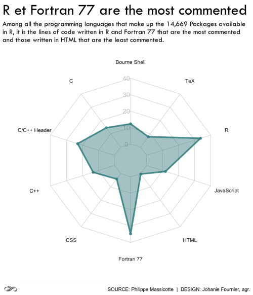
image_annotate("R et Fortran 77 are the most commented",
color = "#000000", size = 62.5, location = "+10+5", font='Tw Cen MT') %>%
image_annotate("Among all the programming languages that make up the 14,669 Packages available\nin R, it is the lines of code written in R and Fortran 77 that are the most commented\nand those written in HTML that are the least commented.",
color = "#000000", size = 29.5, location = "+10+80", font='Tw Cen MT')
#image_browse(titre)
# And bring in a logo
logo_raw<-image_read('~/Documents/ENTREPRISE/Projets R/Logo/Logo_f.once_FFFFFF.png')
logo <- logo_raw %>%
image_scale("x30") %>%
image_background("#FFFFFF", flatten = TRUE) %>%
image_border("#FFFFFF", "10x10")
couleur <- image_read('~/Documents/ENTREPRISE/Projets R/couleur/FFFFFF.png')
backgound <- couleur %>%
image_scale("x20") %>%
image_background("#FFFFFF", flatten = TRUE) %>%
image_border("#FFFFFF", "500x20")
footer<-image_composite(backgound, logo, offset="+0+10") %>%
image_annotate("SOURCE: Philippe Massicotte | DESIGN: Johanie Fournier, agr.",
color = "#000000", size = 20, gravity='northeast', location = "+10+25")
- Posted on:
- November 14, 2019
- Length:
- 2 minute read, 373 words
- Categories:
- rstats tidyverse tidytuesday
- Tags:
- rstats tidyverse tidytuesday