TyT2019W47 - Treemap
By Johanie Fournier, agr. in rstats tidyverse tidytuesday
November 20, 2019
Get the data
nz_bird <- readr::read_csv("https://raw.githubusercontent.com/rfordatascience/tidytuesday/master/data/2019/2019-11-19/nz_bird.csv")
## Rows: 217300 Columns: 4
## ── Column specification ────────────────────────────────────────────────────────
## Delimiter: ","
## chr  (2): vote_rank, bird_breed
## dbl  (1): hour
## date (1): date
##
## ℹ Use `spec()` to retrieve the full column specification for this data.
## ℹ Specify the column types or set `show_col_types = FALSE` to quiet this message.
Explore the data
summary(nz_bird)
##       date                 hour        vote_rank          bird_breed
##  Min.   :2019-10-28   Min.   : 0.00   Length:217300      Length:217300
##  1st Qu.:2019-10-30   1st Qu.:10.00   Class :character   Class :character
##  Median :2019-11-04   Median :13.00   Mode  :character   Mode  :character
##  Mean   :2019-11-03   Mean   :13.66
##  3rd Qu.:2019-11-07   3rd Qu.:18.00
##  Max.   :2019-11-10   Max.   :23.00
Prepare the data
vote <- nz_bird %>%
  filter(!is.na(bird_breed))%>%
  group_by(bird_breed) %>%
  summarise(somme=n(), pourcentage=(somme/sum(somme)*100)) %>%
  ungroup() %>%
  arrange(desc(pourcentage))
Visualize the data
gg<-ggplot(vote, aes(area = pourcentage, fill = bird_breed))
gg<-gg+ geom_treemap(color="white")
gg<-gg+ theme(legend.position="none")
gg <- gg + scale_fill_manual(values=c("#BCBCBC","#BCBCBC","#BCBCBC","#BCBCBC","#B5C2ED","#BCBCBC","#BCBCBC","#BCBCBC","#BCBCBC","#BCBCBC","#4867D4","#BCBCBC","#BCBCBC","#BCBCBC","#BCBCBC","#BCBCBC","#BCBCBC","#BCBCBC","#BCBCBC","#BCBCBC","#BCBCBC","#BCBCBC","#BCBCBC","#BCBCBC","#BCBCBC","#BCBCBC","#BCBCBC","#BCBCBC","#BCBCBC","#BCBCBC","#BCBCBC","#6C85DC","#3658D0","#BCBCBC","#BCBCBC","#BCBCBC","#BCBCBC","#BCBCBC","#BCBCBC","#BCBCBC","#BCBCBC","#BCBCBC","#BCBCBC","#BCBCBC","#BCBCBC","#BCBCBC","#BCBCBC","#BCBCBC","#BCBCBC","#BCBCBC","#BCBCBC","#BCBCBC","#BCBCBC","#BCBCBC","#BCBCBC","#BCBCBC","#BCBCBC","#BCBCBC","#BCBCBC","#BCBCBC","#BCBCBC","#BCBCBC","#BCBCBC","#BCBCBC","#BCBCBC","#BCBCBC","#BCBCBC","#BCBCBC","#BCBCBC","#BCBCBC","#BCBCBC","#BCBCBC","#BCBCBC","#BCBCBC","#BCBCBC","#BCBCBC","#BCBCBC","#BCBCBC","#BCBCBC","#BCBCBC","#BCBCBC","#BCBCBC","#BCBCBC","#BCBCBC","#233985", "#BCBCBC", "#BCBCBC"))
#modifier le thème
gg <- gg + theme(panel.border = element_blank(),
panel.background = element_blank(),
plot.background = element_blank(),
panel.grid.major.x= element_blank(),
panel.grid.major.y= element_blank(),
panel.grid.minor = element_blank(),
axis.line.x = element_blank(),
axis.line.y =element_blank(),
axis.ticks.x = element_blank(),
axis.ticks.y = element_blank())
#ajouter les titres
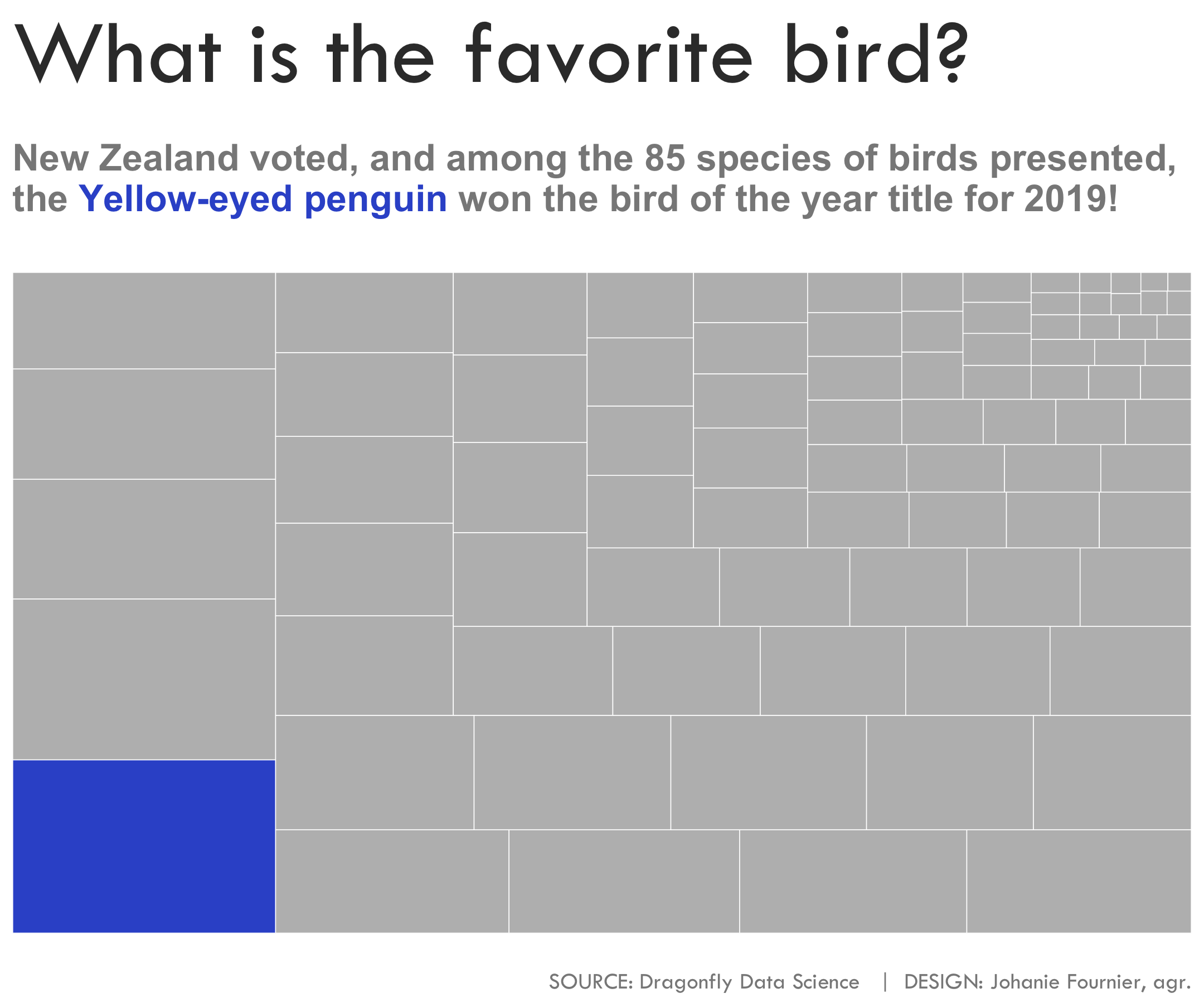
gg<-gg + labs(title="Quels sont les oiseaux favoris?",
subtitle = "<br>La Nouvelle-Zélande a voté et, parmis les 85 espèces d'oiseaux présentés, ce sont<br>le <span style='color:#233985'>**manchot antipode**</span>, le <span style='color:#3658D0'>**perroquet-hibou**</span>, le <span style='color:#4867D4'>**Miro des Chatham**</span>, le <span style='color:#6C85DC'>**Nestor superbe**</span>,<br>le <span style='color:#B5C2ED'>**Pluvier à double collier**</span>, les oiseaux préférés pour l'année pour 2019!<br>",
x=" ",
y=" ",
caption="\nSOURCE: Dragonfly Data Science | DESIGN: Johanie Fournier, agr.")
gg<-gg + theme( plot.title = element_text(size=40, hjust=0,vjust=0.5, family="Tw Cen MT", color="#373737"),
plot.subtitle = element_markdown(lineheight = 1.1,size=16, hjust=0,vjust=0.5, face="bold", color="#898989"),
plot.caption = element_text(size=10, hjust=1,vjust=0.5, family="Tw Cen MT", color="#898989"),
axis.title.y = element_blank(),
axis.title.x = element_blank(),
axis.text.y = element_blank(),
axis.text.x = element_blank())
- Posted on:
- November 20, 2019
- Length:
- 2 minute read, 286 words
- Categories:
- rstats tidyverse tidytuesday
- Tags:
- rstats tidyverse tidytuesday