TyT2020W04 - Visualize Index

Get the data

spotify_songs <- readr::read_csv('https://raw.githubusercontent.com/rfordatascience/tidytuesday/master/data/2020/2020-01-21/spotify_songs.csv')

## Rows: 32833 Columns: 23

## ── Column specification ────────────────────────────────────────────────────────
## Delimiter: ","
## chr (10): track_id, track_name, track_artist, track_album_id, track_album_na...
## dbl (13): track_popularity, danceability, energy, key, loudness, mode, speec...

## 
## ℹ Use `spec()` to retrieve the full column specification for this data.
## ℹ Specify the column types or set `show_col_types = FALSE` to quiet this message.

Explore the data

summary(spotify_songs)

##    track_id          track_name        track_artist       track_popularity
##  Length:32833       Length:32833       Length:32833       Min.   :  0.00  
##  Class :character   Class :character   Class :character   1st Qu.: 24.00  
##  Mode  :character   Mode  :character   Mode  :character   Median : 45.00  
##                                                           Mean   : 42.48  
##                                                           3rd Qu.: 62.00  
##                                                           Max.   :100.00  
##  track_album_id     track_album_name   track_album_release_date
##  Length:32833       Length:32833       Length:32833            
##  Class :character   Class :character   Class :character        
##  Mode  :character   Mode  :character   Mode  :character        
##                                                                
##                                                                
##                                                                
##  playlist_name      playlist_id        playlist_genre     playlist_subgenre 
##  Length:32833       Length:32833       Length:32833       Length:32833      
##  Class :character   Class :character   Class :character   Class :character  
##  Mode  :character   Mode  :character   Mode  :character   Mode  :character  
##                                                                             
##                                                                             
##                                                                             
##   danceability        energy              key            loudness      
##  Min.   :0.0000   Min.   :0.000175   Min.   : 0.000   Min.   :-46.448  
##  1st Qu.:0.5630   1st Qu.:0.581000   1st Qu.: 2.000   1st Qu.: -8.171  
##  Median :0.6720   Median :0.721000   Median : 6.000   Median : -6.166  
##  Mean   :0.6548   Mean   :0.698619   Mean   : 5.374   Mean   : -6.720  
##  3rd Qu.:0.7610   3rd Qu.:0.840000   3rd Qu.: 9.000   3rd Qu.: -4.645  
##  Max.   :0.9830   Max.   :1.000000   Max.   :11.000   Max.   :  1.275  
##       mode         speechiness      acousticness    instrumentalness   
##  Min.   :0.0000   Min.   :0.0000   Min.   :0.0000   Min.   :0.0000000  
##  1st Qu.:0.0000   1st Qu.:0.0410   1st Qu.:0.0151   1st Qu.:0.0000000  
##  Median :1.0000   Median :0.0625   Median :0.0804   Median :0.0000161  
##  Mean   :0.5657   Mean   :0.1071   Mean   :0.1753   Mean   :0.0847472  
##  3rd Qu.:1.0000   3rd Qu.:0.1320   3rd Qu.:0.2550   3rd Qu.:0.0048300  
##  Max.   :1.0000   Max.   :0.9180   Max.   :0.9940   Max.   :0.9940000  
##     liveness         valence           tempo         duration_ms    
##  Min.   :0.0000   Min.   :0.0000   Min.   :  0.00   Min.   :  4000  
##  1st Qu.:0.0927   1st Qu.:0.3310   1st Qu.: 99.96   1st Qu.:187819  
##  Median :0.1270   Median :0.5120   Median :121.98   Median :216000  
##  Mean   :0.1902   Mean   :0.5106   Mean   :120.88   Mean   :225800  
##  3rd Qu.:0.2480   3rd Qu.:0.6930   3rd Qu.:133.92   3rd Qu.:253585  
##  Max.   :0.9960   Max.   :0.9910   Max.   :239.44   Max.   :517810

glimpse(spotify_songs)

## Rows: 32,833
## Columns: 23
## $ track_id                 <chr> "6f807x0ima9a1j3VPbc7VN", "0r7CVbZTWZgbTCYdfa…
## $ track_name               <chr> "I Don't Care (with Justin Bieber) - Loud Lux…
## $ track_artist             <chr> "Ed Sheeran", "Maroon 5", "Zara Larsson", "Th…
## $ track_popularity         <dbl> 66, 67, 70, 60, 69, 67, 62, 69, 68, 67, 58, 6…
## $ track_album_id           <chr> "2oCs0DGTsRO98Gh5ZSl2Cx", "63rPSO264uRjW1X5E6…
## $ track_album_name         <chr> "I Don't Care (with Justin Bieber) [Loud Luxu…
## $ track_album_release_date <chr> "2019-06-14", "2019-12-13", "2019-07-05", "20…
## $ playlist_name            <chr> "Pop Remix", "Pop Remix", "Pop Remix", "Pop R…
## $ playlist_id              <chr> "37i9dQZF1DXcZDD7cfEKhW", "37i9dQZF1DXcZDD7cf…
## $ playlist_genre           <chr> "pop", "pop", "pop", "pop", "pop", "pop", "po…
## $ playlist_subgenre        <chr> "dance pop", "dance pop", "dance pop", "dance…
## $ danceability             <dbl> 0.748, 0.726, 0.675, 0.718, 0.650, 0.675, 0.4…
## $ energy                   <dbl> 0.916, 0.815, 0.931, 0.930, 0.833, 0.919, 0.8…
## $ key                      <dbl> 6, 11, 1, 7, 1, 8, 5, 4, 8, 2, 6, 8, 1, 5, 5,…
## $ loudness                 <dbl> -2.634, -4.969, -3.432, -3.778, -4.672, -5.38…
## $ mode                     <dbl> 1, 1, 0, 1, 1, 1, 0, 0, 1, 1, 1, 1, 1, 0, 0, …
## $ speechiness              <dbl> 0.0583, 0.0373, 0.0742, 0.1020, 0.0359, 0.127…
## $ acousticness             <dbl> 0.10200, 0.07240, 0.07940, 0.02870, 0.08030, …
## $ instrumentalness         <dbl> 0.00e+00, 4.21e-03, 2.33e-05, 9.43e-06, 0.00e…
## $ liveness                 <dbl> 0.0653, 0.3570, 0.1100, 0.2040, 0.0833, 0.143…
## $ valence                  <dbl> 0.518, 0.693, 0.613, 0.277, 0.725, 0.585, 0.1…
## $ tempo                    <dbl> 122.036, 99.972, 124.008, 121.956, 123.976, 1…
## $ duration_ms              <dbl> 194754, 162600, 176616, 169093, 189052, 16304…

Prepare the data

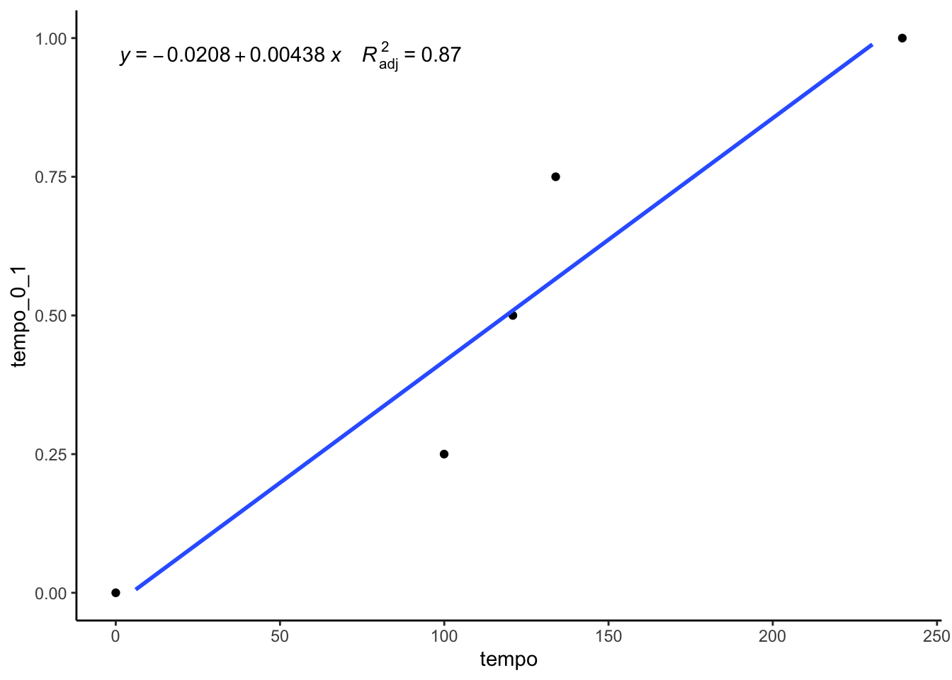
# convertir le tempo en un indicateur qui varie entre 0 et 1
tempo<-data.frame(tempo=c(0,99.96,120.88,133.92,239.44),tempo_0_1=c(0,0.25,0.50,0.75,1))
formula <- y ~ x
gg<- ggplot(data=tempo, aes(x=tempo, y=tempo_0_1))
gg<- gg + geom_point()
gg<- gg + geom_smooth(method='lm', se=FALSE, formula=formula)
gg<- gg +  stat_poly_eq(aes(label =  paste(..eq.label.., ..adj.rr.label.., sep = "~~~~")),
                   formula = formula, parse = TRUE)
gg<- gg + theme_classic()
gg<- gg + scale_y_continuous(limits=c(0,1))
gg

## Warning: Removed 5 rows containing missing values (geom_smooth).

data<-spotify_songs %>% 
  select(playlist_genre, danceability, energy,valence,tempo) %>% 
  mutate(tempo_0_1=0.00438*tempo-0.0208) %>% 
  select(-tempo) %>% 
  gather(type, valeur,-playlist_genre) %>% 
  group_by(playlist_genre, type) %>% 
  summarise_if(is.numeric, median, na.rm = TRUE) %>%
  ungroup() 

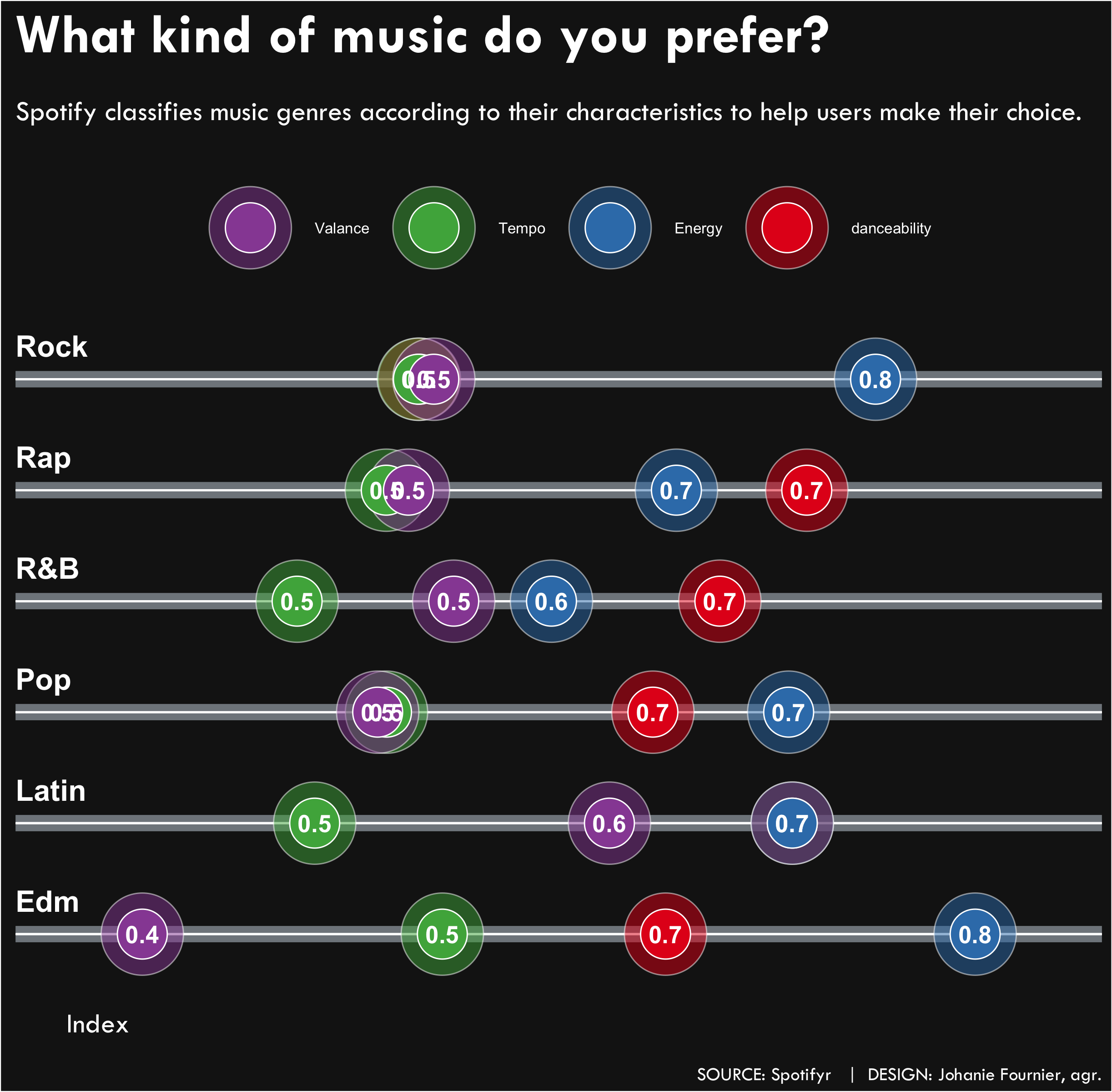
Visualize the data

#Graphique
gg<- ggplot(data=data,aes(x = valeur, y=playlist_genre))
gg <- gg + geom_segment( aes(x=0.3, xend=0.9,y=playlist_genre, yend=playlist_genre),
                           color="#838A90", alpha=0.6, size=4)
gg <- gg + geom_segment( aes(x=0.3, xend=0.9,y=playlist_genre, yend=playlist_genre),
                           color="#ffffff", alpha=1, size=0.5)
gg <- gg +  geom_point(aes(fill=type, group=playlist_genre), color="#FFFFFF", size=20, pch=21, alpha=0.5)
gg <- gg +  geom_point(aes(fill=type, group=playlist_genre), color="#FFFFFF", size=12, pch=21)
gg <- gg + scale_fill_brewer(palette = "Set1",labels=c("danceability","Energy", "Tempo", "Valance"))
#ajouter les étiquettes de points
gg<-gg + geom_text(data=data, aes(x=valeur, y=playlist_genre, label=(round(data$valeur,1)), group=NULL), color="#ffffff", size=4.5, vjust=0.5, hjust=0.5, fontface="bold")
#pour l'axe des y à l'intérieur du graphique
gg<-gg + annotate(geom="text",x=0.3, y=1.3, label="Edm", color="#ffffff", size=5.5, vjust=0.5, hjust=0, fontface="bold")
gg<-gg + annotate(geom="text",x=0.3, y=2.3, label="Latin", color="#ffffff", size=5.5, vjust=0.5, hjust=0, fontface="bold")
gg<-gg + annotate(geom="text",x=0.3, y=3.3, label="Pop", color="#ffffff", size=5.5, vjust=0.5, hjust=0, fontface="bold")
gg<-gg + annotate(geom="text",x=0.3, y=4.3, label="R&B", color="#ffffff", size=5.5, vjust=0.5, hjust=0, fontface="bold")
gg<-gg + annotate(geom="text",x=0.3, y=5.3, label="Rap", color="#ffffff", size=5.5, vjust=0.5, hjust=0, fontface="bold")
gg<-gg + annotate(geom="text",x=0.3, y=6.3, label="Rock", color="#ffffff", size=5.5, vjust=0.5, hjust=0, fontface="bold")
#ajuster l'axe des x
gg <- gg + scale_x_continuous(expand = c(0,0))
#modifier le thème
gg <- gg +  theme(plot.background = element_rect(fill = "#171717"),
                  panel.background = element_rect(fill = "#171717"),
                  panel.grid.major.y= element_blank(),
                  panel.grid.major.x= element_blank(),
                  panel.grid.minor = element_blank(),
                  axis.line.x = element_blank(),
                  axis.line.y =element_blank(),
                  axis.ticks.x = element_blank(), 
                  axis.ticks.y = element_blank())
gg <- gg +  theme(legend.position="top", 
                  legend.title = element_blank(), 
                  legend.background = element_blank(),  
                  legend.key=element_blank(),
                  legend.spacing.x = unit(0.2, 'cm'), 
                  legend.text= element_text(hjust =0.5,size= 8, colour = "#FFFFFF"))
gg <- gg +    guides(fill = guide_legend(nrow = 1, reverse = TRUE))

#ajouter les titres
gg<-gg + labs(title="What kind of music do you prefer?",
            subtitle = "\nSpotify classifies music genres according to their characteristics to help users make their choice.\n",
              x="Index", 
              y=" ", 
              caption="\nSOURCE: Spotifyr   |  DESIGN: Johanie Fournier, agr.")
gg<-gg + theme(  plot.title    =  element_text(size=30, hjust=0,vjust=0.5, color="#FFFFFF", family="Tw Cen MT", face="bold"),
                 plot.subtitle = element_text(size=15, hjust=0,vjust=0.5, color="#FFFFFF", family="Tw Cen MT"),
                 plot.caption  = element_text(size=10, hjust=1,vjust=0.5, color="#FFFFFF", family="Tw Cen MT"),
                 axis.title.x  = element_text(size=15, hjust=0.05,vjust=0.5, color="#FFFFFF", family="Tw Cen MT", angle =0),
                 axis.title.y  = element_blank(),
                 axis.text.y   = element_blank(), 
                 axis.text.x   = element_blank())